The Bayesian Battleship Benchmark (B^3): Evaluating LLM Sequential Decision Making
Motivation
Large language models (LLMs) are increasingly being used across industries for a wide range of tasks. As they become more deeply integrated into technical workflows, it is important to understand how these models behave and when they fail. In many current applications, LLMs operate within a human-in-the-loop process:
- The model proposes an action
- A human accepts or rejects it
- The process repeats, or the human intervenes directly
There are two primary ways this system can break down: either the human’s beliefs/acceptance are miscalibrated, or the model’s proposals are miscalibrated. If the human has incorrect beliefs or acceptance procedures, the process may converge toward poor decisions unless the model consistently proposes strong choices. Conversely, if the model’s outputs are poorly calibrated, it may take many iterations to reach a satisfactory result. This is a familiar experience for many (repeatedly prompting an LLM to generate correct code can take as long as writing it from scratch). This interaction can be viewed as a stochastic sequential decision process, which induces a new distribution over outcomes, defined by the model’s proposal distribution filtered through the human’s acceptance behavior.
While this human-in-the-loop setup provides some safety, there is growing interest in removing the human entirely and allowing LLMs to act autonomously. There are a number of ways this could be done. One approach would be to replace the human filter with some other kind of filter. For example, forcing an LLM’s code to satisfy unit tests could be considered a kind of filter. However, convenient non-human filters are not universally available and in that setting the proposal behavior of the LLM solely drives outcomes.
This raises the question: what kind of sequential decision processes are induced by an LLM? Do LLMs efficiently utilize information when making sequential decisions? These questions are difficult to answer in general, but they can be studied in specific settings. Ideally, we would like a task where we can define a clear notion of rational decision-making and compare model behavior against a principled benchmark.
To explore this, I evaluated several LLMs on their ability to play the game Battleship. Briefly, Battleship is played on a grid where ships of varying lengths are hidden, and the player iteratively selects grid locations to “fire” at, receiving feedback (a hit or a miss) until all ships are sunk. To introduce additional structure, I imposed an additional constraint; ships are not allowed to be adjacent to one another. This significantly reduces the space of valid board configurations, introducing much more information into the problem per move.
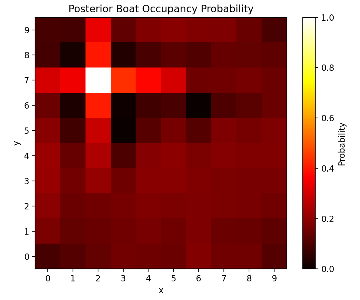
This setting is useful because it allows both performance evaluation by the LLMs and a reasonable method to compare to them. Specifically, I will compare Bayesian strategies of the problem to LLMs. A Bayesian player maintains a posterior distribution over ship placements conditioned on observed hits and misses. Cells that are consistent with many valid ship configurations will have higher posterior probability than those that are not. From the eyes of a Bayesian player, even a few misses contain a lot of information about the board. Below is what the posterior probability of boat occupancy looks like when there are two misses ([3,5], [6,6]) and a hit ([2,7]). Notice how a hit immediately identifies reasonable locations of the ship, but even misses produce “shadows” of decreased probability.
Given this posterior, several reasonable policies emerge:
- Maximum a Posteriori (MAP) - Shoot at the cell most likely to contain a ship.
- Information Gain (Max Marginal Entropy) - Shoot at the cell with the highest posterior entropy.
- Thompson Sampling - Draw a board configuration from the posterior and fire at a ship
- Posterior Draws - Shoot at a draw from a random cell weighted by the posterior probability of it containing a ship.
However, obtaining the exact posterior is computationally challenging due to the combinatorial constraints of the game. To estimate this distribution, I develop an efficient sequential Monte Carlo (SMC) approximation that allows us to estimate a high-quality approximation of the posterior in a reasonable amount of time.
In this work, I compare these probabilistic sequential decision processes enabled by my SMC sampler to those induced by prompting LLMs. I also evaluated the behavior of these LLMs when they were able to select from one of the probabilistic strategies mentioned above each turn. In this setting, the LLMs act as a “coordinator” for well defined policies. In our experiments, LLMs are evaluated without chain-of-thought reasoning and under strict output token limits. These constraints are realistic in many applications (like the current project) where we are sensitive to costs. For this reason, models like Gemini 3.1 Pro were excluded due to the inability to disable thinking and difficulties getting it to conform to constrained JSON scheme output within the token limit. In particular, I analyze:
- GPT 5.4
- Claude Sonnet 4.6
- Gemini Flash 2.5
- Gemma 3 (4B-Q4_K_M)
- LLaMA 3.1 (8B-Q4_K_M)
Results
Policy Comparisons and Gameplay Examples
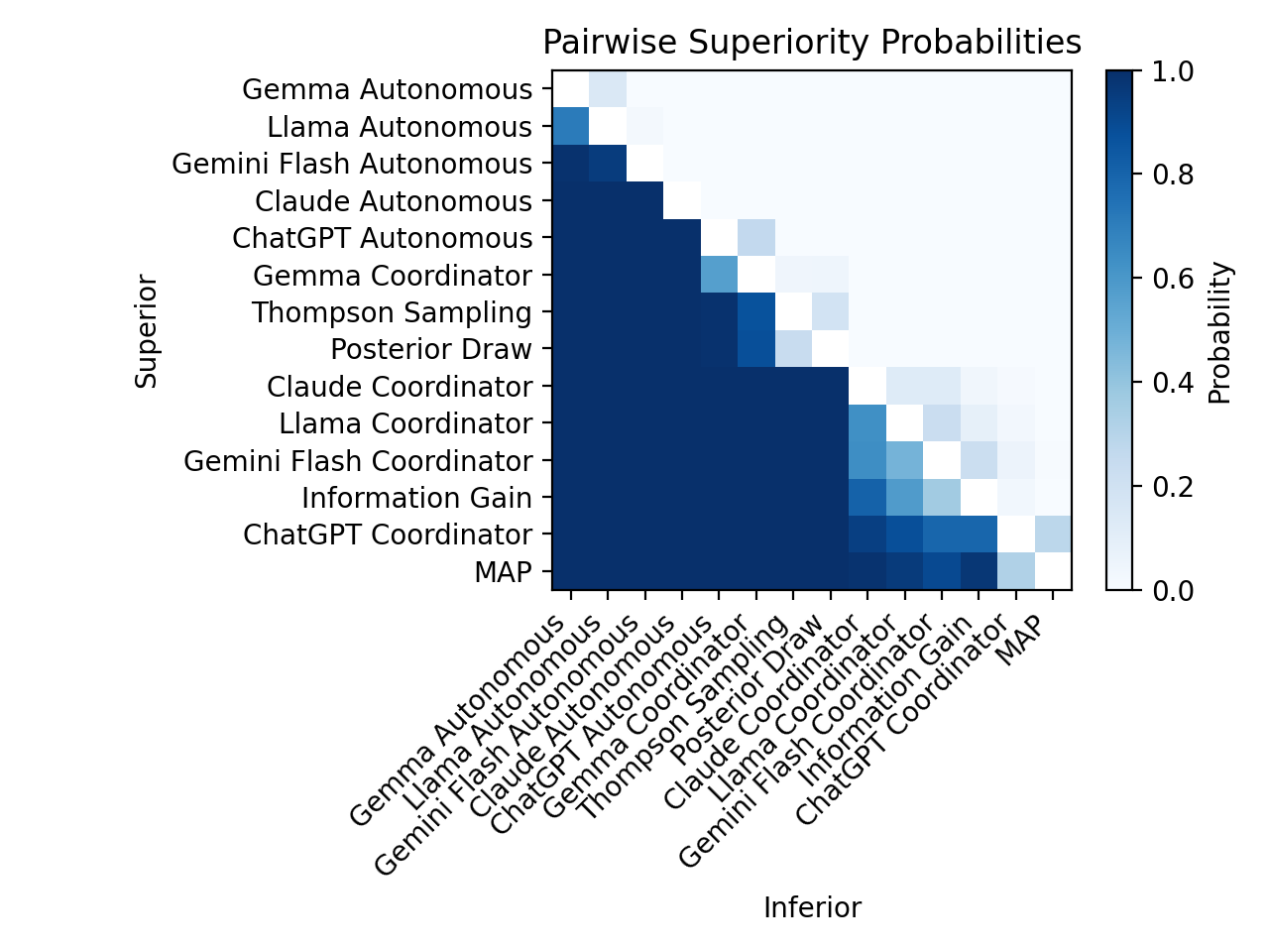
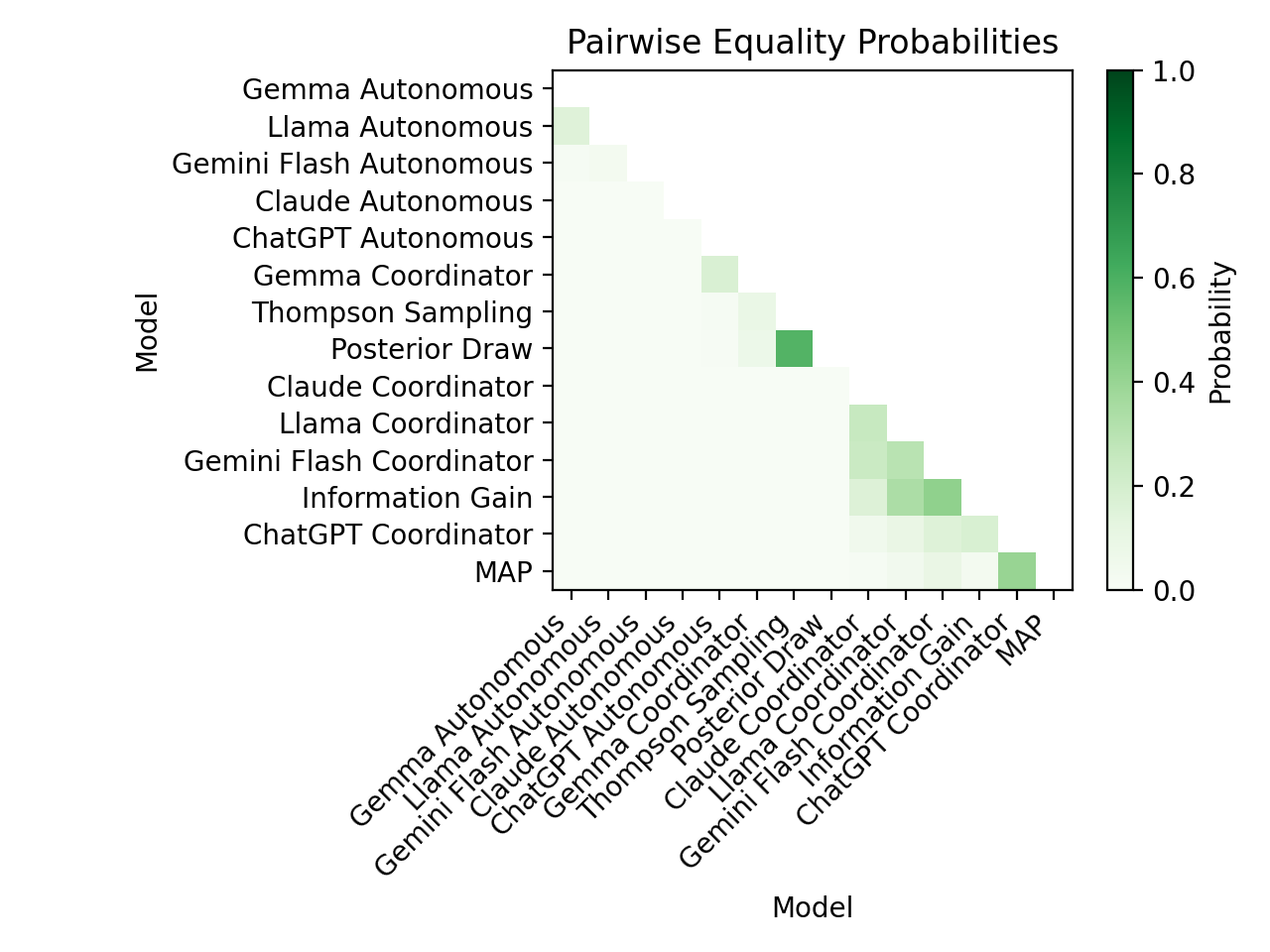
Overall, Bayesian policies outperform all autonomous LLM policies, and LLM-based coordinators largely inherit their performance from the Bayesian strategies they select. Below, the first heatmap shows the probability that one method is strictly superior to another (i.e., wins more than half the time), while the second shows the probability that two methods perform equivalently in a match up.
For each game, we generated animations of gameplay along with per-move metrics. In particular, we tracked posterior deviation and information deviation. Posterior deviation measures how far a player’s move deviates from the MAP action and serves as a measure of exploitative behavior. Information deviation measures how far a move deviates from the action that maximizes information gain, capturing how much the model prioritizes uncertainty reduction. In the animations, I also mark turns resulting in a hit using dashed red lines. Full animations are available on the project’s GitHub. To avoid overcrowding this write-up, here I show a few example animations for the MAP, GPT and Claude policies.
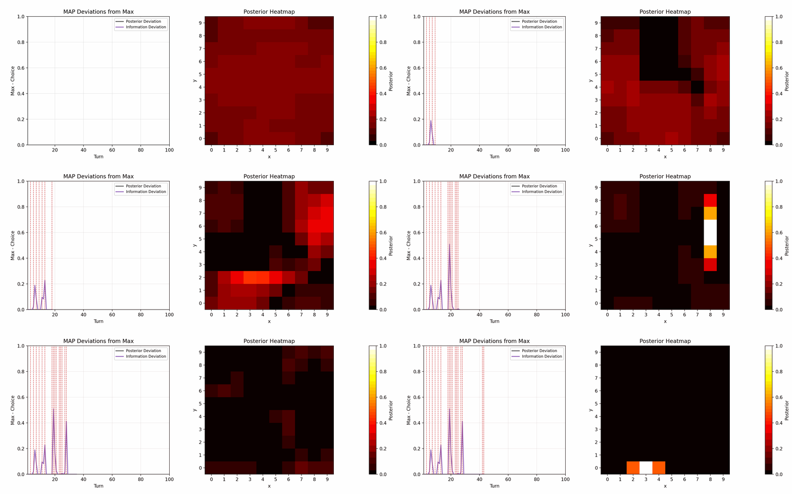
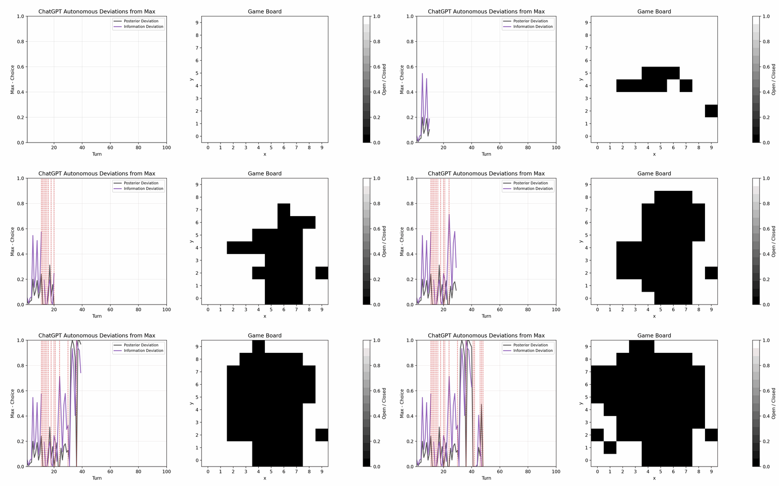
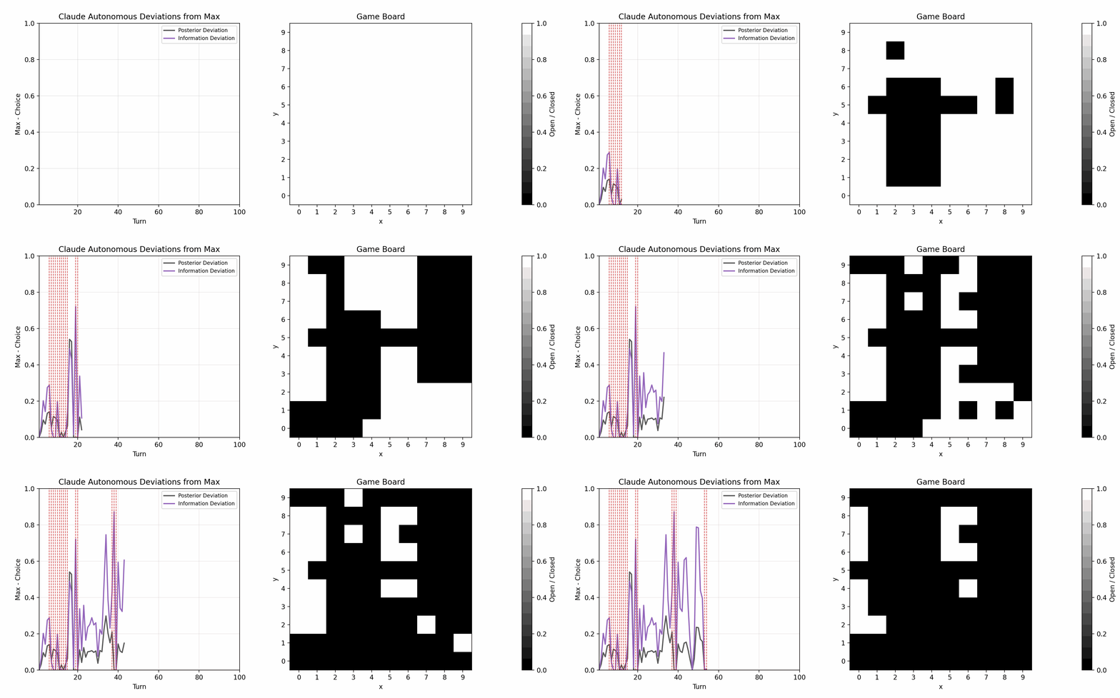
One notable observation is that both GPT and the MAP policy begin with a parity strategy in these games. These strategies exploit the fact that ships must occupy at least two adjacent cells, leading to a checkerboard-style search pattern. For the MAP policy, this behavior emerges naturally from the posterior geometry. For GPT, it is unclear whether this behavior is learned explicitly or arises implicitly from training. Additionally, GPT does not apply this strategy consistently; it appears in many of the games, but GPT will deviate from this strategy, which is observable in the game above.
LLM Rankings
The LLM performance rankings are as follows:
- GPT 5.4
- Claude Sonnet 4.6
- Gemini Flash 2.5
- LLaMA 3.1
- Gemma 3
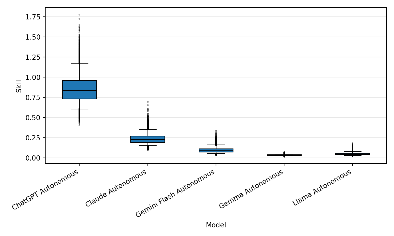
These rankings are based on the posterior medians of a Bradley–Terry model, with posterior skill distributions shown below.
When LLMs exceeded token limits or failed to respond, we assigned a random move as a fallback (described below). Claude autonomous had the highest fallback rate, followed by Gemini Flash autonomous and coordinator. Claude’s fallbacks were primarily due to token overuse. Even with “thinking” disabled, it appeared to generate internal reasoning before producing the required JSON output, exceeding the 196-token limit. Interestingly, the Claude coordinator exhibited no fallbacks, suggesting reduced internal generation when selecting policies rather than actions. Gemini Flash fallbacks were largely due to server-side request failures.
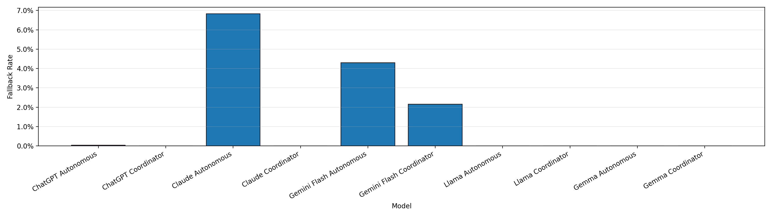
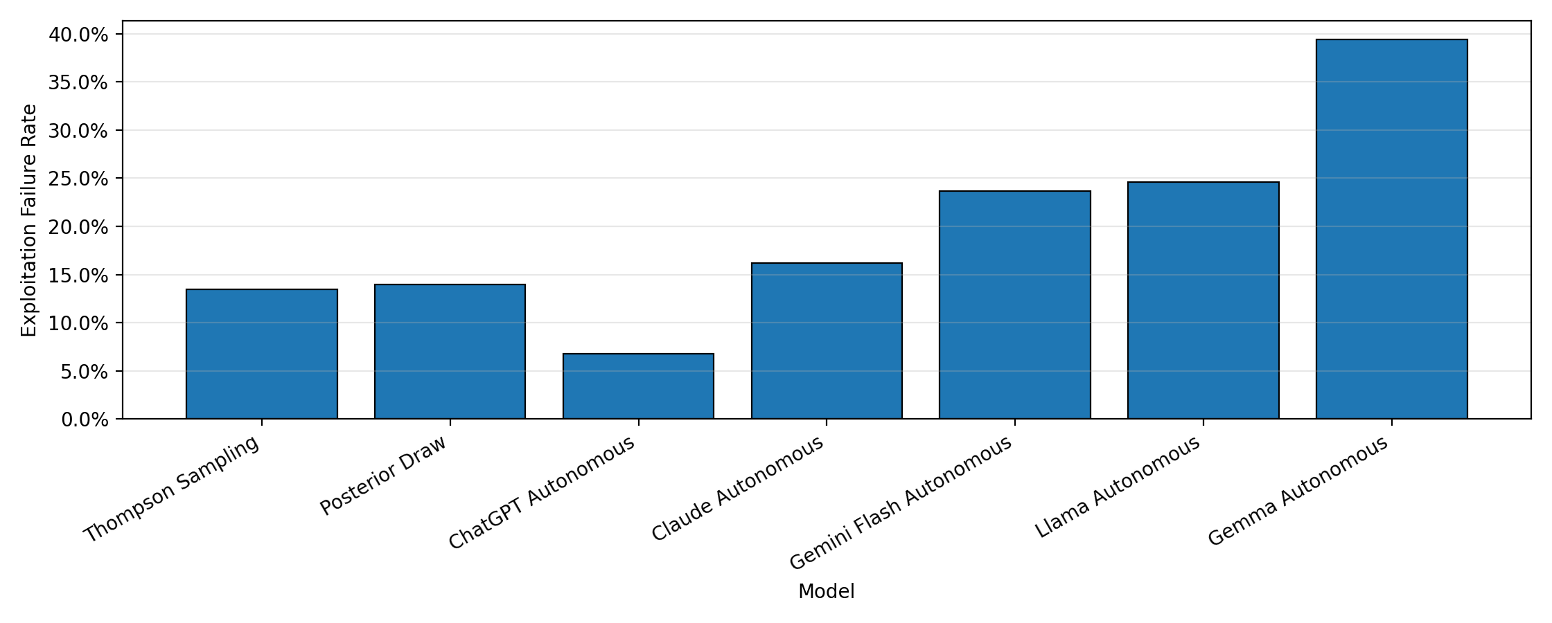
Including fallbacks in our experiments means that the overal performance is a combination of decision quality and service reliability. While fallback rates degrade performance, I don’t believe they substantially alter the ranking. This is supported by exploitation failure rates, defined as the proportion of turns where posterior deviation exceeds 0.75. These correspond to cases where a clearly optimal move exists but is not chosen. Importantly, fallback turns are excluded from this metric. The ranking remains unchanged under this metric, with GPT still performing best.
Completion Distributions
To better understand LLM behavior, I examined their distributions over possible moves. Specifically, I analyzed how their LLM completion distributions compare to the posterior over board states. Note that these represent distributions over different things. The posterior reflects the probability that a ship occupies a cell, while the completion distribution reflects the probability that the model selects that cell. If we idealize what these models are doing internally, the completion distribution can be viewed as the model’s belief about which move is optimal.
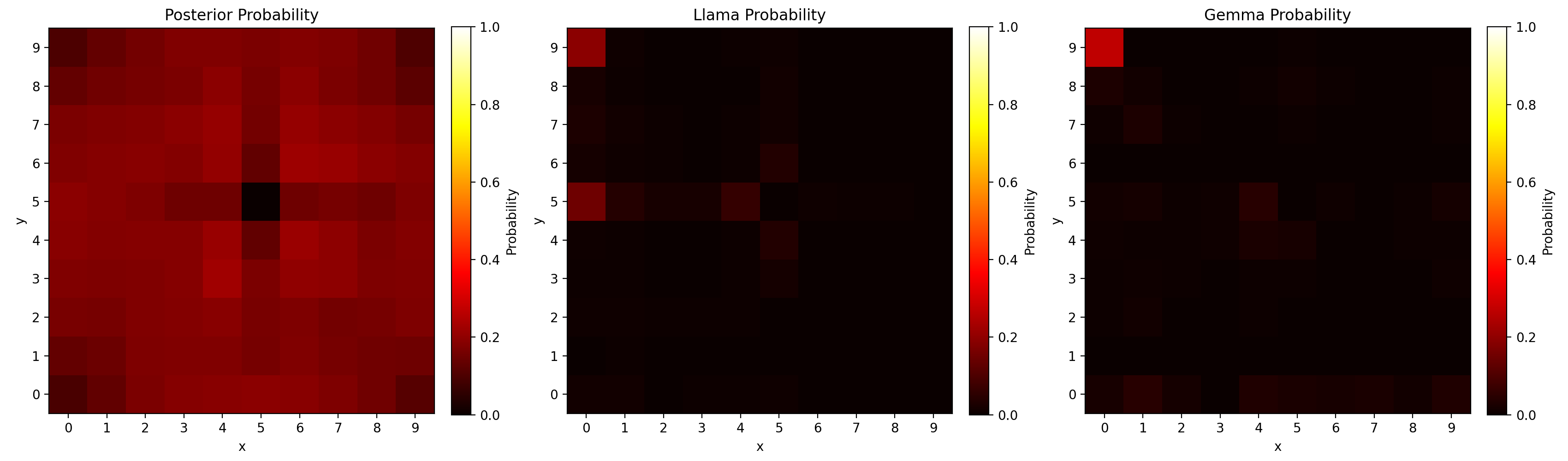
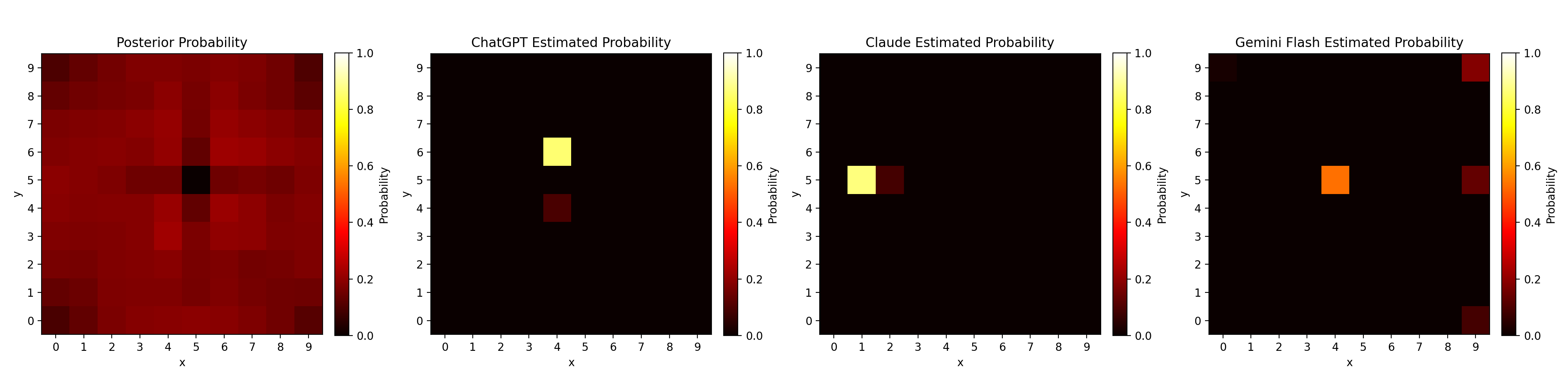
With a single miss on the board (at [5,5]), the posterior assigns lower probability to adjacent cells, as expected. However, the open LLMs behave differently; LLaMA and Gemma assign substantial probability mass to these adjacent cells. Both also show strong bias toward the top-left corner (A1), indicating sensitivity to the ordering of choices (A1 is the first choice provided to them in the list).
API-based models behave differently. Gemini Flash shows biases that do not clearly align with choice ordering and often favors suboptimal adjacent moves. Claude tends to avoid adjacent cells but does not select the strongest options. GPT assigns probability to two high-quality diagonal moves, aligning more closely with the posterior.
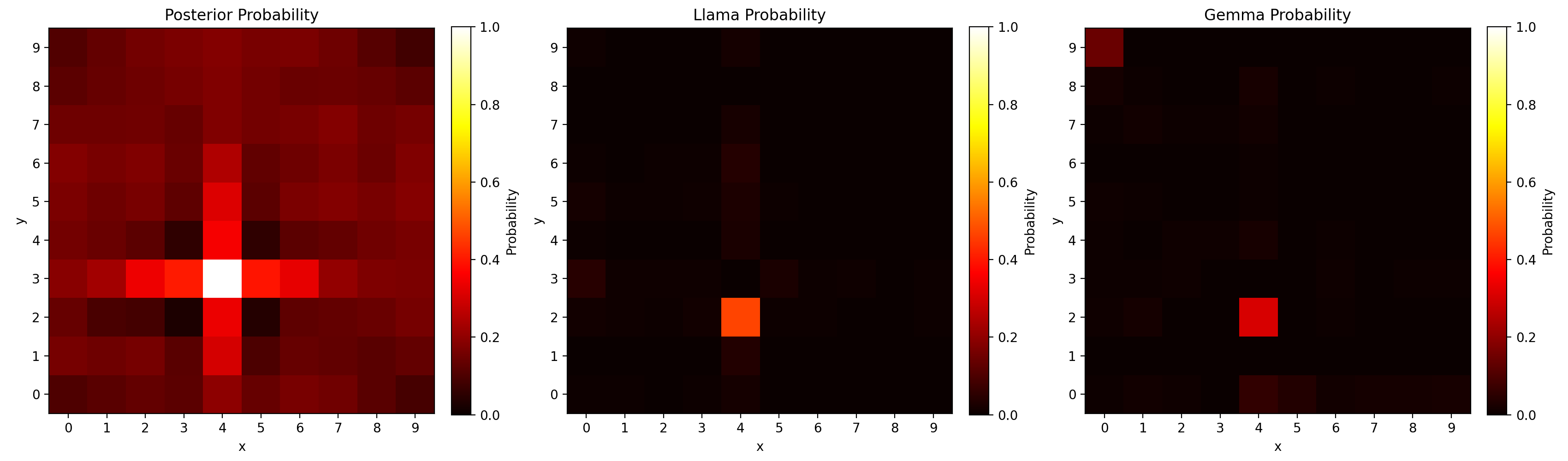
Following a hit (at [4,3]), open models generally assign high probability to reasonable moves but still distribute substantial mass over suboptimal options.
Among API-based models, Claude and GPT concentrate probability on strong moves with relatively low uncertainty, while Gemini Flash distributes probability more broadly across plausible options.
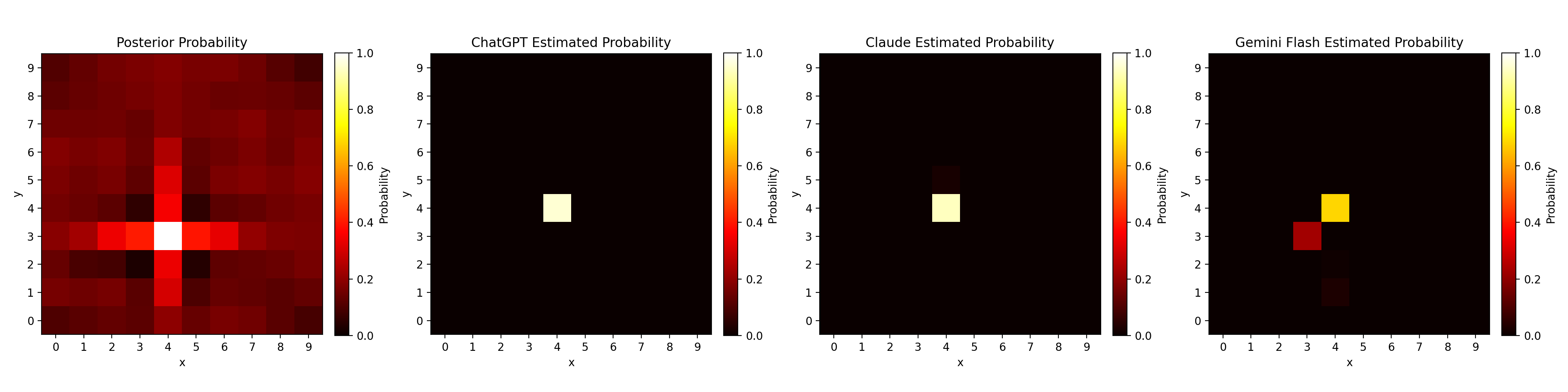
Overall, LLMs perform reasonably well when exploiting hits but struggle to extract useful information from misses. We also empirically see that the completion distributions for API-based models are highly concentrated on a small subset of moves. This suggests that evaluating models under deterministic decoding (temperature set to 0) likely does not substantially alter their behavior, as stochastic sampling would likely select the same high-probability actions.
Coordinator Behavior
We also evaluated LLMs as coordinators selecting among predefined probabilistic policies. In general, coordinator behavior was uninteresting. Most models defaulted to a single strategy rather than combining them meaningfully. Claude and Gemma were exceptions.
Claude exhibited a interesting approach, alternating between exploration and exploitation - using information gain until a hit occurred, then switching to a MAP policy. Gemma was also interesting, initially using posterior sampling before transitioning to information gain. Despite these interesting behaviors, neither approach outperformed the MAP policy, which remained the strongest overall strategy. Below is a histogram showing the proportion of strategies selected by each coordinator.
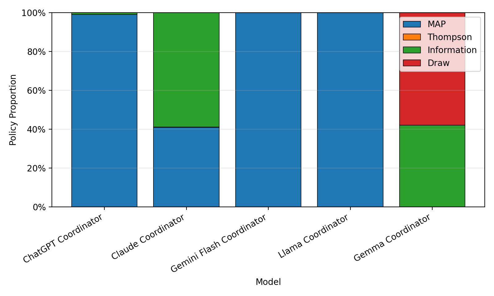
Initially, I anticipated that this might be a strong application of LLMs, with them inducing a kind of routing function over policy primitives. It is moderately surprising to me that this did not turn out to be the case. That being said, it is entirely possible that choosing MAP every turn was really the best choice.
Takeaways
In this work, I investigated the sequential decision-making behavior of LLMs in a setting where the true state of the system is unobserved. While Battleship is a simplified environment, it captures an important feature of many real-world problems - that actions must be chosen under uncertainty, and informative signals are often indirect or negative.
The results show that, in this setting, LLMs tend to underutilize available information, particularly when it arises from indirect feedback. Although performance will certainly vary across domains, this suggests that LLM-based decision processes may be less effective in problems where careful consideration of latent factors is required.
As interest grows in deploying LLMs in more autonomous settings, it is worth considering how such systems will perform in when this kind of inference is required and explicit feedback is limited. Rather than relying solely on LLM outputs, this points to the potential importance of incorporating additional structure into these decision systems, such as probabilistic models, external decision mechanisms or human oversight.
Methodology
Below I describe the methodology I used for these analyses. Note that the exact code and all data/animations from the simulations can be found on my Github for the project.
Posterior Sampling
The posterior distribution over Battleship board configurations is highly combinatorial and constrained by observed hits, sunk ships, and misses. While generating configurations consistent with misses and sunk ships is straightforward, enforcing consistency with partial hits imposes difficult, non-local constraints, particularly when multiple ships are partially observed simultaneously.
To approximate this posterior, I designed a SMC sampler over board configurations. This maintains a population of particles representing candidate boards and introduce hit constraints gradually using an annealing scheme. Initially, particles are required to match known misses and fully sunk ships, but not partial hits. Over successive iterations, configurations inconsistent with observed hits are penalized. At each step, particles are resampled according to their weights and mutated via Metropolis-Hastings proposals, allowing the population to concentrate on configurations consistent with all observations.
I adopt a posterior that consists of a uniform prior over valid board configurations and a likelihood function defined in terms of the number of uncovered incomplete hits. That is, define a board to be \(B = \{(x,y) : x,y \in [1,10]\}\) and the state of each of those cells on that board to be \(f(x,y) \in \{\text{Sunk}, \text{Hit}, \text{Miss}\}\). We say that a ship object is a set of contiguous cells and that given a region of the board \(A \subseteq B\), a ship \(s\) sits on the cells \(A \cap s\). We will denote the whole set of unsunk ships and their placements to be \(S = \{s_1, s_2, \dots\}\), the collection of cells covered by ships to be \(C(S) = \bigcup_is_i\), and the set of hit cells to be \(B^H = ((x,y) \in B : f(x,y) = \text{Hit})\). We adopt the following probability function for an observed board state, given a ship placement \(S\):
\[p(B^H | S)\propto \begin{cases} 1 & \text{if } B^H \subseteq C(S) \\ 0 & \text{otherwise} \end{cases}\]Because it is straightforward to accommodate during sampling, misses and sunk ships are treated as hard constraints that define the support of the prior over configurations, rather than being incorporated into the likelihood.
As it is written, the resulting posterior is extremely peaked, with each board configuration being surrounded by invalid ones in configuration space. This is where our choice of SMC bridging distribution is useful. Rather than trying to sample board configurations that strictly agree with our observations, in SMC, one creates a series of distributions that sequentially get approach our target. In this case, a strong solution is to construct distributions of the form
\[p_\alpha(B^H | S)\propto \alpha^k\]where \(0\leq \alpha \leq 1\) and \(k = \vert B^H\vert - \vert B^H \cap C(S)\vert\) (the number of uncovered hits). By starting our sampler at \(\alpha = 1\) and progressively decreasing it towards \(0\) we create a series of distributions that smoothly approaches our target. If we use a geometric annealing schedule such that \(\alpha_t = \beta \alpha_{t-1}\) we get easily computable unnormalized importance weights, given by \(\beta^{k}\).
This SMC sampler makes estimating posterior probabilities efficient, however it is approximate in a very important way. Notice that it does not account for the information obstained from the fact that the ship is not sunk. This means that board configurations that exactly cover the observed hits are considered valid configurations. While this slightly reduces the posterior probability of neighboring cells, it typically does not alter the ranking of high-probability moves. For example, in the case of two adjacent hits, some posterior mass is assigned to configurations corresponding to a ship of length two occupying those cells exactly. This reduces the posterior probability of extending the ship into adjacent cells, but MAP-based decisions remain unchanged in these scenarios. However, this approximation does result in a more exploitative information-gain policy, which I discuss below.
In all experiments, I use 2,000 particles, 10 SMC iterations, and a geometric annealing schedule with \(\beta = 0.9\).
Bayesian Policies
Using the posterior distribution, I implemented 4 strategies:
- Maximum a Posteriori - Select the cell with the highest posterior probability of containing a ship.
- Information Gain (Max Marginal Entropy) - True information gain would require evaluating the expected reduction in entropy over the full posterior distribution of board configurations for each outcome of a shot, which very computationally expensive. Instead, I use the marginal entropy of each cell as a proxy, selecting moves that maximize local uncertainty. That is, given the marginal posterior probability at a cell \(p_{x,y}\), select the cell that maximizes the entropy \(H(p_{x,y}) = -p_{x,y}\log(p_{x,y}) - (1-p_{x,y})\log(1-p_{x,y})\). I also include a special case when a cell has a probability \(p_{x,y} \geq 0.9\) and select the maximum probability cell when that is the case. This is to prevent edge-cases that could prevent a pure information gain policy from completing the game.
- Thompson Sampling - Draw a configuration from the posterior distribution and target a random boat from that configuration.
- Posterior Draws - Draw a random cell to shoot at, weighted by the posterior probability of it containing a ship.
As mentioned above, the posterior distribution produced by our SMC sampler sometimes produces greater uncertainty in cells that would extend an observed hit. This makes the information gain policy slightly more exploitative than it would be otherwise. For example, consider a scenario where there is only a single cell that would make sense to sink a ship. A pure information gain strategy would not sink that ship because it already knows what is under that cell. Meanwhile, in our sampler, there may be some proportion of the posterior distribution that only perfectly covers the observed hits, not extending into the next logical hit. This induces a greater entropy in the aforementioned cell, encouraging an information gain policy to sink that ship. Note that this behavior can only occur if there are ships available that can perfectly cover the board, which may not be the case over the whole course of a game.
Autonomous LLMs
For LLM-based policies, each move is generated by conditioning the model on the current board state using a structured prompt. The system prompt specifies the rules of the game and the decision task, while the user prompt encodes the current game state, encoded in traditional battlefield coordinates (i.e., A5, F9, etc.):
system_prompt = """
You are playing Battleship (ships are not adjacent).
Select a Battleship target from the provided candidates.
All candidates provided are valid.
"""
prompt = (
        f"Hits on unsunk ships: {hits_text}\n"
        f"Known misses: {misses}\n"
        f"Possible ships remaining: {available_ships}\n"
)
All models are evaluated with temperature set to 0, enforcing greedy decoding, and outputs are constrained to a maximum length of 196 tokens. Setting this temperature to 0 decreases the variance in our estimates and treats the LLMs as optimizing some latent criterion. To ensure parseable outputs, I enforce a JSON schema over completions. An example configuration (for GPT 5.4) is shown below.
payload = {
    "model": OPENAI_MODEL,
    "instructions": system_prompt,
    "temperature": temp,
    "input": prompt,
    "max_output_tokens": DEFAULT_MAX_TOKENS,
    "store": False,
    "text": {
        "format": {
            "type": "json_schema",
            "name": "move_choice",
            "strict": True,
            "schema": {
                "type": "object",
                "properties": {
                    "choice" :{
                        "type": "string",
                        "enum": choices,
                    }
                    },
                "required": ["choice"],
                "additionalProperties": False
            }
        }
    }
}
If an API call fails (e.g., due to token limits or provider-side errors), the system falls back to selecting a random valid move. As a result, measured model performance reflects a combination of reasoning ability and service reliability. Each game of Battleship requires around 50 turns on average in these simulations and required many hours to complete all simulations; therefore I was unable to supervise many of these games and used this fallback as a safety mechanism from generating an unlimited number of token limited failed completions. Empirically, reasoning appears to dominate overall performance (see results above).
Investigating Completion Distributions
To further analyze LLM behavior, I investigated the distribution over possible move completions. For open-weight models such as Gemma and LLaMA, this can be done by explicitly enumerating candidate completions and extracting their logits. Specifically, I construct a prompt that partially pre-fills the expected JSON output format, allowing us to evaluate the likelihood of each valid move under the model. For example, with LLaMA:
prompt_str = (
    "<|begin_of_text|>"
    "<|start_header_id|>system<|end_header_id|>\n"
    f"{system_prompt}<|eot_id|>"
    "<|start_header_id|>user<|end_header_id|>\n"
    f"{prompt}\nYou have the choices: {choices}<|eot_id|>"
    "<|start_header_id|>assistant<|end_header_id|>\n"
    "{'choice': '"
)
Each candidate move is appended to this prefix, and the corresponding logits are computed. These logits are then normalized using a softmax transformation (at temperature 1.0) to obtain an approximate distribution over model completions. Although the choice of temperature here is arbitrary, comparing raw logits has a less intuitive scale and setting the temperature to 0 like I use above does not show the variation in possible action choices.
Although we don’t have access to completion logits in the context of the API-based LLMs, we can still approximate this distribution by sampling completions of the same prompt from the LLM at a temperature of 1.0. Here I do 100 samples per LLM model to estimate this distribution.
Coordinator LLMs
The coordinator policies operate under conditions identical to those of autonomous LLM policies, but utilize the following prompt:
    system_prompt = """
    You are playing Battleship (ships are not adjacent). Choose one strategy for this turn:
        - MAP: Select the cell with the highest posterior probability of containing a ship.
        - THOMPSON: Sample a full board from the posterior, then select a cell from that sample.
        - INFORMATION: Select the cell that maximizes expected information gain.
        - DRAW: Randomly select a cell, weighted by the posterior probability of a hit.
    """
    prompt = (
        f"Hits on unsunk ships: {hits_text}\n"
        f"Known misses: {misses}\n"
        f"Possible ships remaining: {available_ships}\n"
    )
Simulations
To simulate the performance of each policy, I leverage the fact that Battleship does not require player interaction. The game is essentially a race to sink the opponent’s ships. As a result, to estimate the win rate of one policy versus another, we may model the distribution of turns-until-completion for each policy, rather than explicitly simulating every pairwise matchup.
To keep the project within budget, I simulated 50 boards for all policies and computed their turns-until-completion. Because the Bayesian policies incur no additional cost, I simulated an additional 250 boards for those methods to improve precision in their performance estimates.
Since each LLM was evaluated on only 50 games, I decided I should explicitly model uncertainty in downstream analyses. In particular, I use Bayesian bootstrap procedures to produce bootstrap-based posterior distributions over model superiority and latent skill parameters from a Bradley-Terry model.
Given datapoints \(x_1, \dots, x_n\), the Bayesian bootstrap estimates uncertainty in a functional by drawing weights \(w_1, \dots, w_n \sim \text{Dir}(1, \dots, 1)\) and assigning them to each data point. The resulting weighted empirical distribution serves as a proxy for the true data-generating distribution. Repeating this procedure yields a distribution over the functional of interest. Intuitively, this treats some observations as more representative than others and integrates over that uncertainty via Monte Carlo. In my analyses, I used 10,000 bootstrap replicates. We use this approach to generate posterior distributions over turns-until-completion, which then induce posterior distributions over win rates between models.
I also use these Bayesian bootstrap replicates to estimate posterior distributions over latent skill parameters in a Bradley–Terry model. In this setting, the procedure corresponds to a weighted likelihood bootstrap (or loss-likelihood bootstrap), where each replicate computes the maximum likelihood estimate under the weighted data. I use a model of the form:
\[P(A \text{ beats } B) = \frac{e^{\theta_A}}{e^{\theta_A} + e^{\theta_B}}\]I report \(e^{\theta_A}\) as the latent skill of policy \(A\). The model is fit jointly across all pairwise interactions, so the resulting skill estimates reflect aggregate performance across opponents.