Modeling Stochastic Lotka-Volterra using Sequential Neural Likelihood Estimation
Many interesting systems in science can’t be described by closed-form probability distributions. This makes them hard to analyze using classical statistical methods. One common example in biology is the stochastic Lotka–Volterra model, which describes the dynamics of of random predator-prey interactions. It’s a simple model to simulate using the Gillespie algorithm, even though it lacks a closed-form likelihood function.
Briefly, this is how the simulation works:
- Initialize a population of predators (\(a\)) and prey (\(b\)), along with per-capita rates of birth (\(\beta_\text{prey}, \beta_\text{predator}\)), death (\(\gamma_\text{prey}, \gamma_\text{predator}\)), and predation (\(\epsilon\)).
- Compute the event rates:
- Prey birth: \(b \cdot \beta_\text{prey}\)
- Prey death: \(b \cdot \gamma_\text{prey}\)
- Predator birth: \(a \cdot b \cdot \beta_\text{predator}\)
- Predation: \(a \cdot b \cdot \epsilon\)
- Predator death: \(a \cdot \gamma_\text{predator}\)
- Sum all event rates to get the total event rate \(r\), and draw a waiting time \(t \sim \text{Exponential}(r)\).
- Choose an event with probability proportional to its rate (e.g., the probability of predation is \(\frac{a \cdot b \cdot \epsilon}{r}\)), then update the system accordingly.
- Repeat steps 2–4 until a desired simulation time is reached.
Despite being easy to simulate, this model has no closed-form likelihood, which makes traditional parameter estimation difficult. However, if we simulate the model many times under a fixed set of parameters, we get an empirical distribution of likely outcomes, which is essentially a way to score how well different parameters explain the data.
Running millions of simulations for every parameter setting isn’t feasible. Instead, we can train a neural network to approximate this probability distribution based on a finite number of simulations. There are many kinds of these techniques, but here I’ll focus on one: Sequential Neural Likelihood Estimation (SNLE).
SNLE uses normalizing flows to transform a simple base distribution (like a multivariate Gaussian) into one that mimics the complex data-generating process of the simulator. Over successive rounds, the method refines its approximation by focusing simulations on more plausible regions of the parameter space, allowing efficient and accurate inference in models where there is no likelihood. In general, the algorithm looks like this:
- Initialize a prior over parameters, \(P(\theta)\), and an autoregressive conditional normalizing flow (ACNF).
- The ACNF transforms a base multivariate Gaussian into a more flexible distribution using a series of affine transformations. Each transformation is conditioned on the preceding dimensions and parameter values. For more details, see Papamakarios et al. (2018).
- Generate training data by sampling parameter vectors \(\theta\) from the prior \(P(\theta)\) and simulating data from your generative model.
- Train the ACNF to approximate the likelihood \(L_x(\theta)\) based on these parameter–simulation pairs. This gives a crude estimate of the likelihood for the observed data \(x\).
- Run MCMC using the product \(P(\theta) L_x(\theta)\) as the unnormalized posterior. For each sampled \(\theta\), simulate new data under the model.
- Retrain the ACNF on all accumulated parameter–simulation pairs, including both prior samples and MCMC-based samples. This improves the likelihood approximation in regions of high posterior density.
- Repeat steps 4–5 until the ACNF has adequately learned the likelihood in the relevant region of the parameter space.
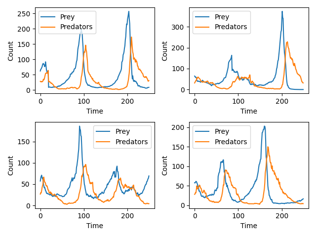
I spent some time earlier this year trying to understand these methods and so I thought I would share a project of mine on the blog. Although I am unsure what I would use this method for in my own research, it is such a clever application of MCMC that I couldn’t help but implement it. The code below trains a conditional autoregressive flow neural network to learn an autoregressive multiplicative random walk that produces Lotka-Volterra dynamics. While Papamakarios et al. (2019) model the full trajectory as a static vector, I chose to model the incremental dynamics autoregressively. This better respects the sequential structure of the Lotka–Volterra system and allows the learned flow to generate new trajectories step-by-step. Below is an image of a four draws from the trained conditional autoregressive flow; the positions and magnitude of the oscillations shown below are a classic Lotka-Volterra pattern. Although I will not print the output here, SNLE also does a pretty good job at inferring the true parameter value of many of my test simulations.
conditional_autoregressive_flow.py
import tensorflow as tf
from tensorflow import keras
import tensorflow_probability as tfp
import matplotlib.pyplot as plt

tfd = tfp.distributions

class ConditionalAutoregressiveFlow(keras.Model):
    """
    A neural network that autoregressively applies affine transformations to an N dimensional
    normal distribution conditional on some provided parameter. Rather than doing masking like in
    masked autoregressive flows, we are just explicitly enforcing the autoregressive nature of the
    network in the structure of the network itself.
    """
    def __init__(self, num_params, num_dimensions, num_flows, internal_dim=16, lr=1e-2):
        super(ConditionalAutoregressiveFlow, self).__init__()
        self.optimizer = tf.keras.optimizers.Adam(learning_rate=lr, clipnorm=1.0)
        self.num_params = num_params
        self.num_dimensions = num_dimensions
        self.internal_dim = internal_dim
        self.num_flows = num_flows

        self.autoregressive_networks = []
        for n in range(num_flows):
            permutation = tf.random.shuffle(tf.range(0, num_dimensions, dtype=tf.int32))
            if(n > 0):
                while tf.math.reduce_all(permutation == self.autoregressive_networks[-1]["permutation"]): # We want to make sure each layer is different from the last
                    permutation = tf.random.shuffle(tf.range(0, num_dimensions, dtype=tf.int32))
            network = []
            for i in range(num_dimensions):
                network.append({
                    "dense": keras.layers.Dense(internal_dim, activation="relu"),
                    "alpha": keras.layers.Dense(1, activation="softplus",kernel_initializer=tf.keras.initializers.RandomNormal(mean=0.5, stddev=0.1, seed=None)),
                    "beta": keras.layers.Dense(1, activation="linear", kernel_initializer=tf.keras.initializers.RandomNormal(mean=0.0, stddev=1.0, seed=None)),
                })
            self.autoregressive_networks.append({"network": network, "permutation": permutation})

        self.base_dist = tfd.MultivariateNormalDiag(loc=tf.ones([num_dimensions]))

    def call(self, flow_input):
        """Normalizing Direction"""
        conditionals = flow_input[:, :self.num_params]
        data = flow_input[:, self.num_params:]
        tf.debugging.assert_equal(data.shape[1], self.num_dimensions,
                                  f"Error: {self.num_dimensions} dimensions of data were expected, but we only got {data.shape[1]}")

        output_list = [data[:, i] for i in range(self.num_dimensions)]

        jacobian_sum = 0
        for n in range(self.num_flows):
            temp_conditionals = conditionals

            network_obj = self.autoregressive_networks[n]
            autoregressive_network = network_obj["network"]
            network_permutation = network_obj["permutation"]

            for i in range(self.num_dimensions):
                index = network_permutation[i]
                y = output_list[index]
                flow = autoregressive_network[index]

                x = flow["dense"](temp_conditionals)
                alpha = tf.squeeze(flow["alpha"](x))
                beta = tf.squeeze(flow["beta"](x))
                y = tf.divide(y - beta, alpha)

                output_list[index] = y
                temp_conditionals = tf.concat([temp_conditionals, tf.expand_dims(y, axis=-1)], axis=-1)

                jacobian_sum += tf.math.log(alpha)

        output = tf.stack(output_list, axis=-1)

        log_prob = self.base_dist.log_prob(output)
        log_prob -= jacobian_sum

        return log_prob

    def transform(self, flow_input):
        """Generative Direction"""
        conditionals = flow_input[:, :self.num_params]
        data = flow_input[:, self.num_params:]

        tf.debugging.assert_equal(data.shape[1], self.num_dimensions,
                                  f"Error: {self.num_dimensions} dimensions of data were expected, but we only got {data.shape[1]}")


        output_list = [data[:, i] for i in range(self.num_dimensions)]


        for n in range(self.num_flows-1, -1, -1):
            temp_conditionals = conditionals

            network_obj = self.autoregressive_networks[n]
            autoregressive_network = network_obj["network"]
            network_permutation = network_obj["permutation"]

            for i in range(self.num_dimensions):
                index = network_permutation[i]
                y = output_list[index]
                flow = autoregressive_network[index]

                x = flow["dense"](temp_conditionals)
                alpha = tf.squeeze(flow["alpha"](x))
                beta = tf.squeeze(flow["beta"](x))
                y = tf.multiply(y, alpha) + beta

                temp_conditionals = tf.concat([temp_conditionals, tf.expand_dims(output_list[index], axis=-1)], axis=-1)
                output_list[index] = y

        output = tf.stack(output_list, axis=-1)

        return output

    def draw(self, parameters, num_draws = 1):
        """Generative Direction"""
        conditionals = tf.tile(tf.expand_dims(parameters, axis=0), [num_draws,1])
        data = self.base_dist.sample(num_draws)
        flow_input = tf.concat([conditionals, data], axis=-1)

        return self.transform(flow_input)


    def train_step(self, data):
        """Negative log-likelihood loss"""

        with tf.GradientTape() as tape:
            log_likelihood = self(data)
            loss = -tf.reduce_mean(log_likelihood)

        trainable_vars = self.trainable_variables
        gradients = tape.gradient(loss, trainable_vars)

        self.optimizer.apply_gradients(zip(gradients, trainable_vars))

        return {"loss": loss}

if __name__=="__main__":
    scale = tf.random.uniform([500], 4.0, 8.0, dtype=tf.float32)
    scale = tf.reshape(tf.repeat(scale, 1000), [-1])
    quandrant_flag = tfd.Bernoulli(0.5, dtype=tf.bool).sample(scale.shape[0])
    mean_vec = tf.where(quandrant_flag, scale * -1.0, scale)
    training_samples = tf.squeeze(tfd.MultivariateNormalDiag([mean_vec, mean_vec*-1]).sample(1))
    training_input = tf.concat([tf.expand_dims(scale, axis=-1), tf.transpose(training_samples)], axis=-1)

    test_af = ConditionalAutoregressiveFlow(num_params = 1, num_dimensions = 2, num_flows = 5, internal_dim = 64)

    losses = []
    for i in range(500):
        loss = test_af.train_step(training_input)['loss']
        losses.append(loss)
        print(f"Loss at Epoch {i}: {loss}")

    transformed_data = test_af.draw([5.5], num_draws=1000)

    dummy_data = tfd.MultivariateNormalDiag(loc=tf.ones([2])).sample(1000)
    dummy_data_input = tf.concat([tf.fill([dummy_data.shape[0], 1], 7.5), dummy_data], axis=-1)
    transformed_data_2 = test_af.transform(dummy_data_input)

    fig1, ax1 = plt.subplots()
    ax1.scatter(x = transformed_data[:, 0], y = transformed_data[:, 1], label="Scale = 5.5", alpha=0.5)
    ax1.scatter(x = transformed_data_2[:, 0], y = transformed_data_2[:, 1], label="Scale = 7.5", alpha=0.5)
    ax1.legend()
    ax1.set_ylabel("Y")
    ax1.set_xlabel("X")
    ax1.set_title("Transformation")
    fig1.savefig("./conditional_af_transformation.png")

    x_min = -10
    x_max = 10
    y_min = -10
    y_max = 10
    num_x = 100
    num_y = 100

    x = tf.linspace(x_min, x_max, num_x)
    y = tf.linspace(y_min, y_max, num_y)

    X, Y = tf.meshgrid(x, y)
    coordinates = tf.stack([tf.reshape(X, [-1]), tf.reshape(Y, [-1])], axis=-1)
    coordinates = tf.cast(coordinates, tf.float32)

    coordinate_input = tf.concat([tf.fill([coordinates.shape[0], 1], 7.5), coordinates], axis=-1)
    probs = tf.math.exp(test_af(coordinate_input))
    heatmap = tf.reshape(probs, (num_y, num_x))

    fig2, ax2 = plt.subplots()
    ax2.imshow(heatmap.numpy(), extent=[x_min, x_max, y_min, y_max], origin='lower', cmap='viridis')
    ax2.set_ylabel("Y")
    ax2.set_xlabel("X")
    ax2.set_title("Transform Probability")
    fig2.savefig("./conditional_af_pdf.png")
sequential_neural_likelihood_lotka_volterra.py
import tensorflow as tf
from tensorflow import keras
import tensorflow_probability as tfp
import matplotlib.pyplot as plt
from conditional_autoregressive_flow import ConditionalAutoregressiveFlow
import math

tfd = tfp.distributions

class LogConditionalAutoregressiveFlow(ConditionalAutoregressiveFlow):
    """
    Our conditionals interact on a multiplicative scale, and we are
    modeling a multiplicative random walk - so our neural network should
    reflect that. We log transform all of our conditionals to express that.
    """
    def call(self, flow_input):
        """Normalizing Direction"""
        conditionals = tf.math.log(flow_input[:, :self.num_params])
        data = tf.math.log(flow_input[:, self.num_params:])
        tf.debugging.assert_equal(data.shape[1], self.num_dimensions,
                                  f"Error: {self.num_dimensions} dimensions of data were expected, but we only got {data.shape[1]}")

        output_list = [data[:, i] for i in range(self.num_dimensions)]

        # Adjust for the log transform (-1 * log(original data))
        jacobian_sum = -1 * tf.reduce_sum(data, axis=-1)
        for n in range(self.num_flows):
            temp_conditionals = conditionals

            network_obj = self.autoregressive_networks[n]
            autoregressive_network = network_obj["network"]
            network_permutation = network_obj["permutation"]

            for i in range(self.num_dimensions):
                index = network_permutation[i]
                y = output_list[index]
                flow = autoregressive_network[index]

                x = flow["dense"](temp_conditionals)
                alpha = tf.squeeze(flow["alpha"](x))
                beta = tf.squeeze(flow["beta"](x))
                y = tf.divide(y - beta, alpha)

                output_list[index] = y
                temp_conditionals = tf.concat([temp_conditionals, tf.expand_dims(y, axis=-1)], axis=-1)

                jacobian_sum += tf.math.log(alpha)

        output = tf.stack(output_list, axis=-1)

        log_prob = self.base_dist.log_prob(output)
        log_prob -= jacobian_sum

        return log_prob

    def transform(self, flow_input):
        """Generative Direction"""
        conditionals = tf.math.log(flow_input[:, :self.num_params])
        data = flow_input[:, self.num_params:]

        tf.debugging.assert_equal(data.shape[1], self.num_dimensions,
                                  f"Error: {self.num_dimensions} dimensions of data were expected, but we only got {data.shape[1]}")


        output_list = [data[:, i] for i in range(self.num_dimensions)]

        for n in range(self.num_flows-1, -1, -1):
            temp_conditionals = conditionals

            network_obj = self.autoregressive_networks[n]
            autoregressive_network = network_obj["network"]
            network_permutation = network_obj["permutation"]

            for i in range(self.num_dimensions):
                index = network_permutation[i]
                y = output_list[index]
                flow = autoregressive_network[index]

                x = flow["dense"](temp_conditionals)
                alpha = tf.squeeze(flow["alpha"](x))
                beta = tf.squeeze(flow["beta"](x))
                y = tf.multiply(y, alpha) + beta

                temp_conditionals = tf.concat([temp_conditionals, tf.expand_dims(output_list[index], axis=-1)], axis=-1)
                output_list[index] = y

        output = tf.stack(output_list, axis=-1)

        return tf.math.exp(output)


def generative_model(prey_birth, predation, predator_birth, predator_death, init_predators=30, init_prey=60, total_time=100, samples_per_unit_time=5):
    """
    Simulate a time series of stochastic Lotka-Volterra dynamics.
    Here we will output the multiplicative increase from the previous step.
    """

    # Enforce minimum for simplicity
    prey_birth = prey_birth + 1e-2
    predation = predation + 1e-2
    predator_birth = predator_birth + 1e-2
    predator_death = predator_death + 1e-2

    times = [0.0]
    predators = [init_predators]
    prey = [init_prey]

    while True:
	    # Get current population
        prey_count = prey[-1]
        predator_count = predators[-1]

		# Determine event rates
        prey_birth_rate = prey_birth*prey_count
        predation_rate =  predation*prey_count*predator_count
        predator_death_rate = predator_death*predator_count
        predator_birth_rate = predator_birth*predator_count*prey_count

		# Get total "race" rate
        total_rate = prey_birth_rate + predation_rate + predator_death_rate + predator_birth_rate
        if(total_rate == 0): # Total extinction
            break

        # These are what we based the uniform draw on
        prey_birth_cumulative = prey_birth_rate/total_rate
        predation_cumulative = predation_rate/total_rate + prey_birth_cumulative
        predator_death_cumulative = predator_death_rate/total_rate + predation_cumulative

        waiting_time = tfd.Exponential(total_rate).sample(1)

        new_time = times[-1] + waiting_time
        if(new_time < total_time):
            times.append(new_time)
            # Draw a random event (birth, death, predation)
            action_draw = tf.random.uniform([1], 0.0, 1.0)
            if(action_draw < prey_birth_cumulative):
                predators.append(predator_count)
                prey.append(prey_count + 1.0)
            elif(action_draw < predation_cumulative):
                predators.append(predator_count)
                prey.append(prey_count - 1.0)
            elif(action_draw < predator_death_cumulative):
                predators.append(predator_count - 1.0)
                prey.append(prey_count)
            else:
                predators.append(predator_count + 1.0)
                prey.append(prey_count)
        else:
            break

    time_sampled_prey = []
    time_sampled_predator = []

    increment = 1/samples_per_unit_time
    for i in range(total_time * samples_per_unit_time):
        last_event = 0
        for t in range(len(times)):
            if(times[t] <= i * increment):
                last_event = t
            else:
                break

        time_sampled_predator.append(predators[t])
        time_sampled_prey.append(prey[t])

    current_dim = tf.stack([time_sampled_predator, time_sampled_prey], axis=-1)
    prev_dim = tf.roll(current_dim, shift=1, axis=0)

    # Now we get the increase
    multiplicative_increase = tf.math.divide(current_dim, prev_dim)
    multiplicative_increase = tf.where(tf.math.is_nan(multiplicative_increase), 1e-6, multiplicative_increase)
    multiplicative_increase = tf.where(multiplicative_increase <= 0, 1e-6, multiplicative_increase)
    prev_dim = tf.where(prev_dim == 0, 1e-6, prev_dim)

    # Roll moves the last element to the first, so we shave that off
    output = tf.concat([prev_dim, multiplicative_increase], axis=-1)[1:, :]

    return output

def parameter_update(parameter):
    param_choice = tf.random.uniform([1], 0, 4, dtype=tf.int32) # Pick random param
    param_choice = tf.reshape(param_choice, [1, 1])

    scaler = tf.math.exp(2.0 * tf.random.uniform([1], 0, 1) - 0.5)

    updated_value = parameter[param_choice[0, 0]] * scaler

    parameter = tf.tensor_scatter_nd_update(parameter, param_choice, updated_value)

    return parameter, tf.math.log(scaler)

def mcmc(data, prior, likelihood = None, iterations = 1000, debug = True, sample_iter = 1000):
    """
    If a likelihood is not passed we will do Metropolis Hastings
    on the prior alone. For now we are just going to be doing scale moves
    on the parameter when it comes to working with the product of the prior
    and model. For the prior alone we will just draw directly from the prior.
    This function the final state of the Markov chain, which can be plugged
    into the generative model.
    """
    return_params = []

    if(likelihood is None):
        for i in range(int(iterations/sample_iter)):
            param = tf.squeeze(prior.sample())
            if(debug):
                tf.print(f"Drawing parameter from prior: {param}")
            return_params.append(param)
    else:
        param = tf.squeeze(prior.sample())
        old_posterior = tf.reduce_sum(prior.log_prob(param)) +  tf.reduce_sum(likelihood(tf.concat([tf.tile(tf.expand_dims(param, axis=0), [data.shape[0], 1]), data], axis=-1)))
        for i in range(1, iterations+1):
            new_param, hastings = parameter_update(param)
            new_posterior = tf.reduce_sum(prior.log_prob(new_param)) + tf.reduce_sum(likelihood(tf.concat([tf.tile(tf.expand_dims(new_param, axis=0), [data.shape[0], 1]), data], axis=-1)))
            posterior_ratio = hastings + new_posterior - old_posterior

            draw = tf.random.uniform([1], 0, 1)
            if(tf.math.log(draw) < posterior_ratio):
                param = new_param
                old_posterior = new_posterior
                if(debug):
                    tf.print(f"Accepted new parameter value at iteration {i}: {param}")

            if(i % sample_iter == 0):
                return_params.append(param)

    return return_params


def train_flow_model(training_input, settings, debug = True):
    model = LogConditionalAutoregressiveFlow(settings["num_params"],
    settings["num_dimensions"], settings["num_flows"], settings["internal_dim"], lr=1e-3)

    patience = 25
    min_delta = 1e-2
    best_loss = float('inf')
    waited_epochs = 0

    losses = []
    for i in range(settings["training_iterations"]):
        loss = model.train_step(training_input)['loss']
        losses.append(loss)
        if(debug):
            tf.print(f"Loss at Epoch {i}: {loss}")

        if(loss < best_loss - min_delta):
            best_loss = loss
            waited_epochs = 0
        else:
            waited_epochs += 1

        if(waited_epochs >= patience):
            if(debug):
                tf.print(f"Stopping early at epoch {i}")
            break

    return model

def snle_step(data, prior, model, settings):
    training_data_list = []
    training_param_list = []

    for n in range(settings["num_mcmc_chains"]):
        param = mcmc(data, prior, model, settings["mcmc_iterations"])
        for i in range(settings["num_simulations"]):
            for y in param:
                t_data = generative_model(y[0], y[1], y[2], y[3], total_time = 10, samples_per_unit_time = 10)
                training_param_list.append(y)
                training_data_list.append(t_data)

    return training_param_list, training_data_list

if __name__ == "__main__":
    settings = {"num_params": 6, "num_dimensions": 2,
                "num_flows": 3, "internal_dim": 64,
                "num_retrainings": 4, "num_simulations": 5,
                "num_mcmc_chains": 100, "mcmc_iterations": 2000,
                "training_iterations": 2500}

    training_data_list = []
    training_param_list = []

    model = None
    prior = tfd.Exponential(rate = [4, 20, 20, 4])
    observed_data = generative_model(0.75, 0.01, 0.01, 1.0,
                                    init_predators = 30, init_prey = 60, total_time = 25, samples_per_unit_time = 10)
    print("We generated:")
    print(observed_data)

    for i in range(settings["num_retrainings"]):
        param, data = snle_step(observed_data, prior, model, settings)

        for d in data:
            training_data_list.append(d)
        for p in param:
            training_param_list.append(tf.tile(tf.expand_dims(p, axis=0), [99,1])) # 99 time samples per param because one is sliced off

        training_data = tf.concat(training_data_list, axis=0)
        training_param = tf.concat(training_param_list, axis=0)

        training_input = tf.concat([training_param, training_data], axis=-1)

        model = train_flow_model(training_input, settings)

    fig, axes = plt.subplots(2,2)

    for n, ax in enumerate(axes.flat, start=1):
        param_input = tf.constant([0.75, 0.01, 0.01, 1.0, 60.0, 30.0], dtype=tf.float32)
        prey_counts = [60.0]
        predator_counts = [30.0]
        for i in range(250):
            next_step = model.draw(param_input, num_draws=1)
            predator = max(1e-6, next_step[0, 0].numpy() * predator_counts[-1])
            prey = max(1e-6, next_step[0, 1].numpy() * prey_counts[-1])

            predator_counts.append(predator)
            prey_counts.append(prey)

            param_input = tf.constant([0.75, 0.01, 0.01, 1.0, predator, prey], dtype=tf.float32)

        ax.plot(prey_counts[1:], label="Prey")
        ax.plot(predator_counts[1:], label="Predators")
        ax.set_ylabel("Count")
        ax.set_xlabel("Time")
        ax.legend()

    fig.tight_layout()
    fig.savefig("./lotka_volterra_trajectories.png")